Microbursts, Queuing, and Network Simulation with the Poisson Probability Distribution
Curse of the Microburst
Networks live entire lives in the fraction of a second. Despite this fact, most network metrics are reported in seconds, and it’s usually either a 1 minute or 5 minute average. So if you have a link that is completely saturated for 30s and completely empty for 30s, your metrics tell you it was 50% saturated for that minute. Microbursts are bursts of network traffic that happen at the microsecond level. You and your tools have no hope for observing these without throwing an ungodly amount of resources at it. Your link gets saturated and starts dropping packets, TCP congestion control mechanisms engage, UDP traffic is lost forever, and then people call and complain that their phone calls and streaming videos are choppy. You go look at your trusty graphs, and they show you that your link wasn’t even saturated, which is a lie. You curse the gods and your networking vendor, and then go tell the users to just let you know if it happens again.
Queuing Delay
There are a handful of different types of delay that affect network traffic. Delay is important to understand since it directly affects how much TCP throughput you can achieve. TCP works by sending some packets to a destination, then waiting for an acknowledgement of those packets, and then sending some more. The longer a sender has to wait on acknowledgements, the lower the throughput will be. Queuing delay is how long a packet stays in the buffers of network devices between a source and a destination. Network devices have queues so that they can handle some amount of bursting without dropping packets and triggering TCP congestion control, which will wreck your throughput. There are many different types of queuing mechanisms such as FIFO, Priority Queue, and Active Queuing Mechanisms (AQM). In order to understand queuing mechanisms and their contribution to network delay, it’s important to model and simulate networks correctly.
What is Poisson?
Poisson is a type of probability distribution that tells you the probability of some kind of outcome. In our case, we are going to examine whether Poisson is useful to model how many packets arrive at a port per second. If the average packets per second is 1000 for example, then at any particular second we may see exactly 1000 packets arrive or we could see a different number. Maybe 1050 arrived, or 950, or some other number. Packet arrivals are random like that, but over time they may follow a pattern which could be Poisson.
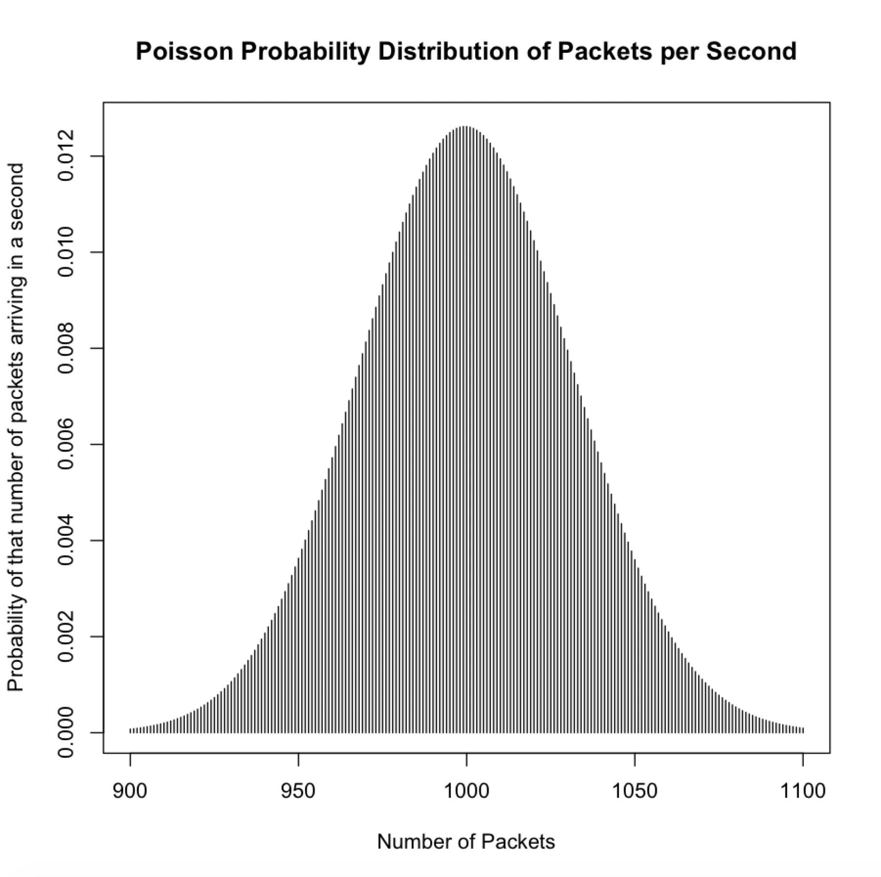
This is a hypothetical histogram of packet arrivals as a Poisson distribution. As can be seen above, the probability of exactly 1000 packets arriving in a second are a little more than 1.2%. The values around 1000 are also pretty close to 1.2% but decrease as packets increase or decrease. Around 900 and 1100 they are pretty close to 0. However, whether real network traffic will follow Poisson remains to be seen.
Note:
A useful property of Poisson is that if a system has a Poisson arrival rate with an average of λ then the interarrival time follows the Exponential Probalility Distribution with mean of 1/λ. The interarrival time is the time between packets. We can therefore test for Poisson by comparing a histogram of packet interarrival times to the exponential distribution to see if it fits.
Measuring an Actual Network Link
So to see if Poisson is actually useful for network modeling, I took a packet capture of a server link. Here is a breakdown of the packet types by port.
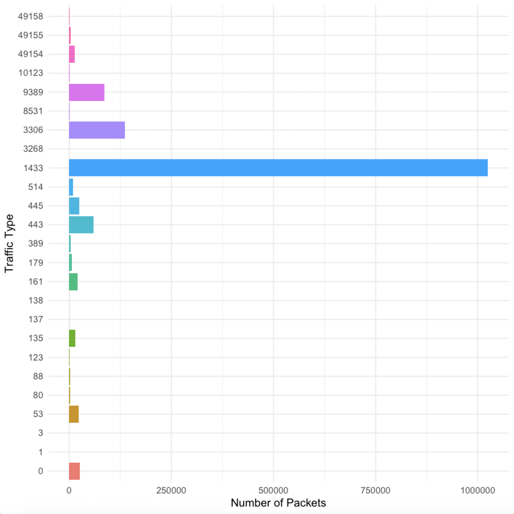
As you can see, port 1433 dominated the packets, which is SQL Server. Another big one is port 3306, which is MariaDB. Port 0 is how I coded ICMP traffic, which doesn’t have a port. I was surprised to see so few packets on port 445, which is windows file sharing or SMB. There is a big file server behind this link, but an important thing to note is that number of packets doesn’t necessarily correspond to amount of data. SQL Server could be sending a lot of small packets while the file server sends a smaller amount of larger packets.
Next, I graphed a histogram of packet interrarrival times to see if it followed the exponential distribution, but this graph was basically unreadable. There was a huge spike near 0, but also a long, flat, heavy tail that reached out to about 3.5 seconds. This happened because the vast majority of packet interarrival times were in the microseconds or even nanoseconds, but there were still a lot of large interarrival times due to lulls between flows. So for kicks, I decided to cut off the heavy tail where it really flattened out, which was about .002s. Here is the histogram of measured arrival times below .002s vs. the exponential distribution with the mean of the measured arrival times below .002s:
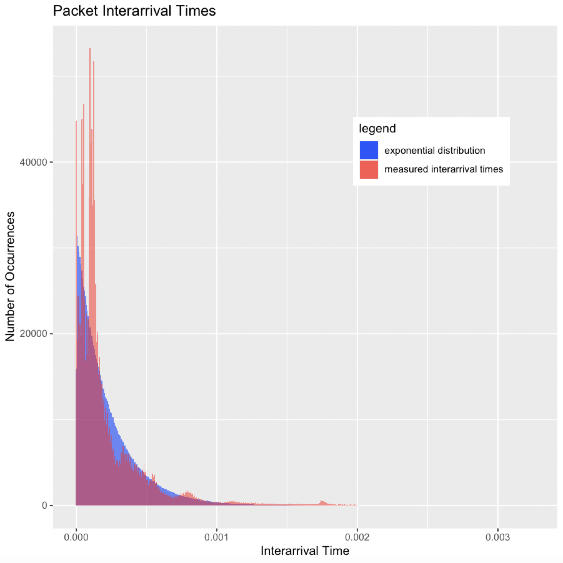
Using a sophisticated statistical test known as “eyeballing it,” the measured packet interarrival times do seem to follow the exponential curve with some caveats. First, I cut off the heavy tail of course. Second, there are a few peaks and valleys that go above and below the exponential curve. This effect is known as multimodality. These peaks and valleys are caused by bursts and lulls of packet arrivals related to flows. Packets on a network are not independent; they are part of flows which are sessions between senders and receivers. Packets that are part of the same flow will have short interarrival times, and if a link has a burst of flows at once, then total packet interarrival times will be even shorter. These bursts show up as the peaks on our chart. Conversely, there may also be lulls between flows on a link which show up as the valleys on our chart.
Is Poisson Appropriate for Network Modeling?
Yes, at least for this traffic in particular, and only if we address the two caveats mentioned above:
- We’re trying to model a network in order to evaluate queuing delay. Will cutting off the heavy tail affect our evaluation? No, in our case, we are primarily concerned with microbursts that saturate a link, so cutting off the heavy tail is okay.
- To address bursts and lulls, we can vary our interarrival rate as we run our simulation. Instead of just keeping the interarrival rate fixed as an exponential with mean 1/λ, we can change lambda throughout the simulation causing packets to arrive much closer together or farther apart thus creating bursts and lulls. I did not do any analysis of a pattern among the peaks and valleys, but in the simulation I modeled the changing λ with a uniform random distribution. Bursts and lulls in a Poisson process are called Poisson Clumping, and I’ve included a resource in the Credits section that details more sophisticated techniques of modeling them.1
If we needed the heavy tail, we could try some other techniques to account for it in our model such as using the Pareto distribution or using self-similarity. Pareto is similar to exponential, but it has a heavier tail. I tried out a plot of the Pareto distribution, and it fit the heavy tail of our data better, but it did not fit the primary section of our histogram very well. Self-similarity is a technique that assumes that a small part of our data is similar to a large part. For example, a graph over microseconds of network traffic will be similar to a graph of seconds or longer time periods. I did not do any analysis for self-similarity, but I have included some resources in the Credits section below that talk more about these techniques.23
Simulating a Network to Evaluate FIFO vs. Priority Queuing
- First-in, First out (FIFO) is typically the default queuing mechanism for switchport buffers unless QoS is setup.
- A Priority Queue gives certain subsets of traffic a better priority that allows it to move through the queue faster.
- Our goal is to simulate how each different queuing mechanism contributes to queuing delay in a network.
- 10 simulations each of 1s were performed.
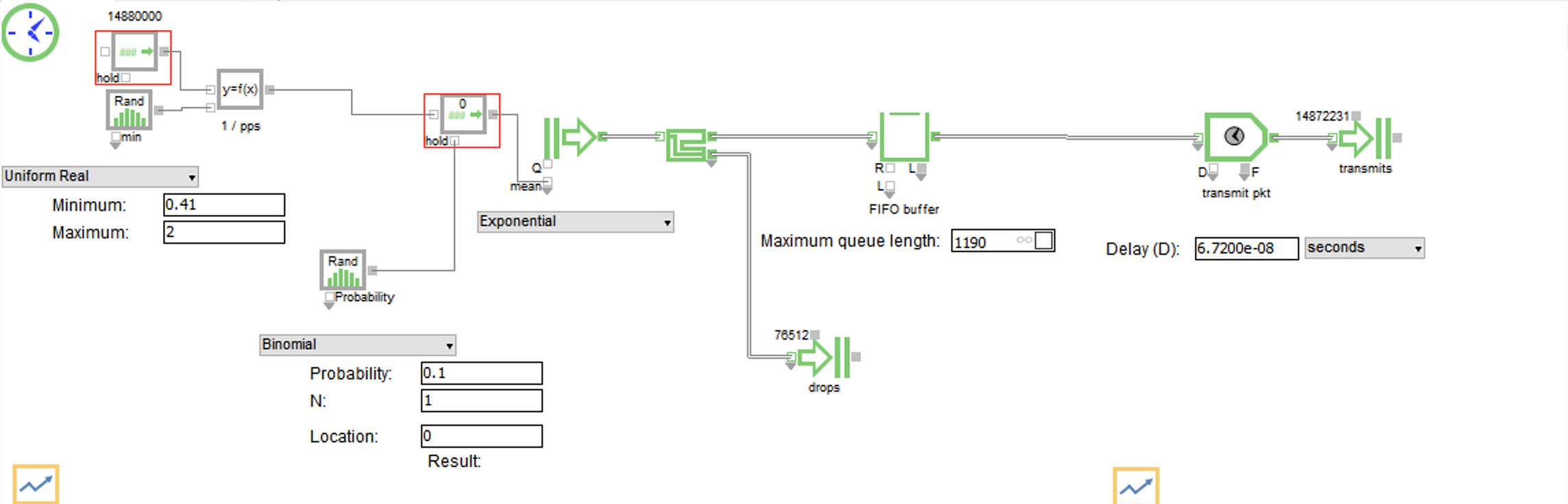
Here is the FIFO buffer:
-
Max packets per second for a 10G port is 14,880,000 64 byte packets or 84 byte ethernet frames. This is used as λ in our simulation. We multiply this factor by random numbers between .41 and 2 that are generated according to a Uniform Real Distribution. This is done to create bursts and lulls in the Poisson arrival rate, and it corresponds to the magnitude of the burst. Maybe the most interesting part of this simulation was coming up with the range to use here. I originally tried a range from 0-2, but this resulted in 0 packets dropped based on the queue length. Through trial and error, I arrived at .41 as the spot where we start to see drops. Having a range of .41-2 means that the port is always receiving at least 6,100,800 packets per second (pps). The λ created with this calculation is inverted to create our 1/λ mean interarrival rate to feed our exponential distribution.
-
Before feeding our exponential distribution, we use a random numbers generated according to a Binomial distribution to govern whether to update the mean interarrival rate on our exponential distribution. This is done to simulate the length of the burst. For clarification, at each step of the burst, there is a 90% chance the interarrival rate will stay the same, and a 10% chance it will stay the same. For multiple steps, you multiply the probabilities. For example, for a burst to last for 5 steps, the probability is .95 which is 59%. It is important to state that this methodology isn’t based on actual analysis of burst length. It was just something I tried that seemed to work well enough for the simulation. In general it seems like there hasn’t been a lot of research on burst length, or at least I wasn’t able to find much.
-
Next is our packet generator, which is the icon in the diagram with a right arrow and two vertical lines behind it. It will create packets according to an exponential distribution with a mean interarrival rate fed from our calculation.
-
After that is our FIFO buffer. The queue length of the FIFO buffer is 1190, and if the queue is full then it will drop packets. The queue length was taken from an Arista article that said that their top-of-rack (TOR) switches have 100KB buffer per 10G port so 100KB/84B = 1190 frames.4
-
After the buffer, the port has to serialize the data onto the wire. This is called transmission delay, and is calculated as 1s/14,880,000pps = 6.72e-8s to send one frame.
Here is the Priority Queue:
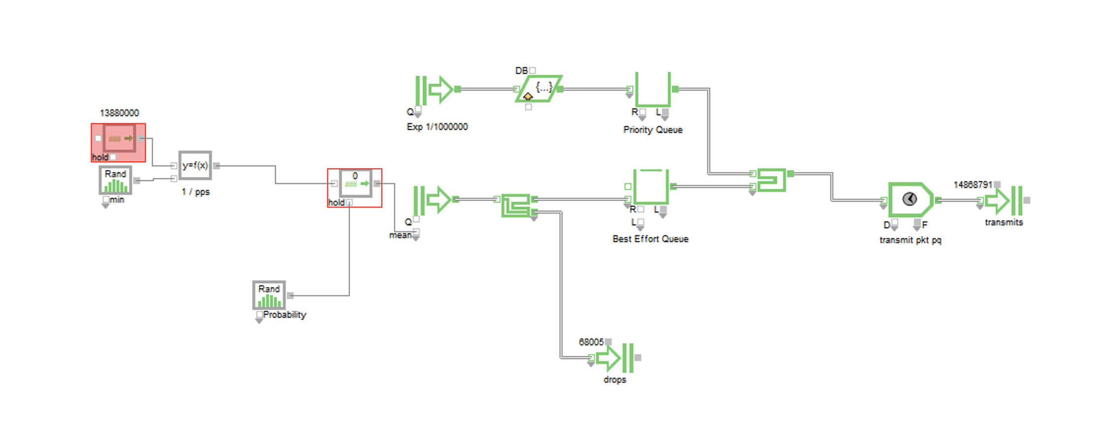
- The Priority queue works exactly like the FIFO queue except now there is a steady 1,000,000pps generated of priority traffic with exponential interarrival times. The port will transmit packets from the priority queue before the best effort queue.
Results
| Block Name | Block | Ave Length | Max Length | Ave Wait | Max Wait |
|---|---|---|---|---|---|
| Best Effort Queue | Queue | 746.5±18.52 | 1190±0.000 | 5.383e-05±1.332e-06 | 8.826e-05±1.898e-07 |
| FIFO buffer | Queue | 733.3±19.65 | 1190±0.000 | 4.932e-05±1.314e-06 | 7.997e-05± |
| Priority Queue | Queue | 0.03598±4.211e-05 | 4.100±0.2262 | 3.600e-08±2.932e-11 | 2.569e-07±1.082e-08 |
These numbers are 95% confidence intervals, which means that if we did this same exact simulation 100 times and computed 100 confidence intervals, 95 of them should contain the “right” number and 5 of them won’t. For the sake of analysis, we’ll assume the ones we have here contain the right value, but there is a chance they don’t.
Unsurprisingly, the priority queue had no drops and the lowest average and max queue wait times. The best effort queue alongside the priority queue had the worst. Both simulations had roughly the same number of total packets dropped, but the FIFO queue had a little bit more.
Takeaways
- If we are concerned with lowest queuing delay for all traffic, we might choose the FIFO queue.
- If we have some traffic that must be prioritized and can’t be dropped, we would choose the Priority queue with the caveat that the rest of the traffic will have longer delay.
- More analysis on burst occurence, magnitude, and length is needed for a better model.
- Packets are part of flows, so simulation and modeling based on flows as the fundamental unit instead of packets might be better.
- More analysis on different traffic profiles is needed to see if Poisson is useful in the general case.
- Knowing your baseline traffic rate and burst range will help you find how big of a buffer you would need to avoid dropping packets.
Note:
The best way to avoid dropped packets and queuing delay is to not have the problem in the first place. Queuing and dropping happens when links are oversubscribed, which means the traffic traversing the link may be greater than what the link can handle. If your links are not oversubscribed, then you will not have a microburst problem or a queuing delay problem. If you can afford bigger links or more links then you should get them. All of this detailed statistical analysis can be be avoided by just throwing money and hardware at the problem. This is why modern datacenters are designed to be non-blocking, which means capacity in = capacity out.
Comments